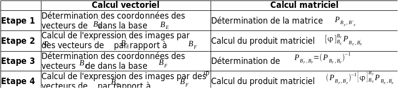
Tableau comparatif des calculs vectoriels et des calculs matriciels
En revenant à l'approche élémentaire du problème posé, il apparaît que les calculs vectoriels qui y sont faits et les calculs matriciels qui interviennent dans ce théorème peuvent être menés en parallèle. Un tableau nous permet de visualiser cette remarque.
Exemple :
Soit\( \phi\) l'application linéaire du \(\mathbf R\)-espace vectoriel\( \mathbf R^3\) dans le \(\mathbf R\)-espace vectoriel \(\mathbf R^2\) définie par \(\phi((x,y,z))=(x+2y+,x-2y+z)\).
Le triplet \((f_1,f_2,f_3)\) avec \(f_1=(1,1,1),f_2=(1,1,0),f_3=(1,0,0)\) est une base de \(\mathbf R^3\), notée \(\mathcal B_f\) (la vérification est immédiate). De même le couple \((\epsilon_1,\epsilon_2)\) avec \(\epsilon_1=(1,1)\) et \(\epsilon_2=(1,0)\) est une base, notée\( \mathcal B_{\epsilon}\), de\( \mathbf R^2\). On se propose de déterminer la matrice de \(\phi\) par rapport aux bases \(\mathcal B_f\) et \(\mathcal B_{\epsilon}\), soit \([\phi]_{\mathcal B_f}^{\mathcal B_{\epsilon}}\) .
Pour cela on va passer par l'intermédiaire des bases canoniques de \(\mathbf R^3\) et de \(\mathbf R^2\) \(\mathcal B=(e_1,e_2,e_3)\) et \(\mathcal B'=(e'_1,e'_2)\) respectivement et utiliser la formule :
\([\phi]_{\mathcal B_f}^{\mathcal B_{\epsilon}}=(\mathcal P_{\mathcal B',\mathcal B_{\epsilon}})^{-1}[\phi]_{\mathcal B}^{\mathcal B'}\mathcal P_{\mathcal B,\mathcal B_f}\).
D'après la définition de \(\phi,\phi(e_1)=(1,1),\phi(e_2)=(2,-2)\) et \(\phi(e_3)=(0,1)\).
Donc la matrice associée à \(\phi\) par rapport aux bases canoniques est \(\left(\begin{array}{cccccc}1&2&0\\1&-2&1\end{array}\right)\).
La matrice de passage de la base \(\mathcal B\) à la base \(\mathcal B_f\) est égale à \(\left(\begin{array}{cccccc}1&1&1\\1&1&0\\1&0&0\end{array}\right)\).
La matrice de passage de la base \(\mathcal B'\) à la base \(\mathcal B_{\epsilon}\) est égale à \(\left(\begin{array}{cccccc}1&1\\1&0\end{array}\right)\).
Comme on a
\(\displaystyle{\begin{array}{cccccc}\epsilon_1&=&e'_1+e'_2\\\epsilon_2&=&e'_1\end{array}}\)
il vient immédiatement
\(\displaystyle{\begin{array}{cccccc}e'_1&=&&\epsilon_2\\e'_2&=\epsilon_1&-&\epsilon_2\end{array}}\)
D'où \((\mathcal P_{\mathcal B',\mathcal B_{\epsilon}})^{-1}=\left(\begin{array}{cccccc}0&1\\1&-1\end{array}\right)\)
Alors \(\displaystyle{[\phi]_{\mathcal B_f}^{\mathcal B_{\epsilon}}=\left(\begin{array}{cccccc}0&1\\1&-1\end{array}\right)\left(\begin{array}{cccccc}1&2&0\\1&-2&1\end{array}\right)\left(\begin{array}{cccccc}1&1&1\\1&1&0\\1&0&0\end{array}\right)}\)
et donc \([\phi]_{\mathcal B_f}^{\mathcal B_{\epsilon}}=\left(\begin{array}{cccccc}0&-1&1\\3&4&0\end{array}\right)\).