Les propriétés du champ magnétostatique

La loi de Biot et Savart permet d'exprimer le champ magnétostatique élémentaire \(\stackrel{\hookrightarrow}{\mathrm{d}B}(M)\) créé en un point \(\mathsf{M}\) par un élément \(I\overrightarrow{\mathrm{d}l}(P)\) de la distribution de courant pris en un point \(\mathsf{P}\) quelconque de \(\mathfrak{(D)}\), soit :

\(\stackrel{\hookrightarrow}{\mathrm{d}B} = \frac {\mu_0}{4\pi} I\overrightarrow{\mathrm{d}l}(P) \wedge \frac{\overrightarrow{PM}}{PM^3}\)

Le produit vectoriel \(I\overrightarrow{\mathrm{d}l}(P) \wedge \frac{\overrightarrow{PM}}{PM^3}\) indique que le champ élémentaire \(\stackrel{\hookrightarrow}{\mathrm{d}B}\) est orthoradial ;

on peut donc écrire \(\stackrel{\hookrightarrow}{\mathrm{d}B} = \mathrm{d}B_{\phi}(M)\vec e_{\phi}\).

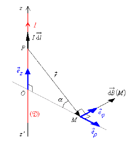
Chacun des vecteurs étant explicité dans la base cylindrique \(\mathfrak{B} = (\vec e_{\rho}, \vec e_{\phi}, \vec e_z)\) :

\(I\overrightarrow{\mathrm{d}l} = I {\displaystyle{ \left( \begin{array}{c c c} 0 \\ 0\\ \mathrm{d}z\end{array}\right)}_{\mathfrak B}}\) et \(\frac{\overrightarrow{PM}}{PM^3} = \frac{1}{PM^3} {\displaystyle{ \left(\begin{array}{c c c} r \cos \alpha  \\ 0\\ -r \sin \alpha \end{array}\right)_{\mathfrak B}}}\)

en effet,

\(\overrightarrow{PM}=\overrightarrow{PO}+\overrightarrow{OM}=\vec r\)

\(\overrightarrow{PO} = -z \vec e_z = -r \sin \alpha \vec e_z\)

\(\overrightarrow{OM} = \rho \vec e_{\rho} = r \cos \alpha \vec e_{\rho}\)

On a : \(I\overrightarrow{\mathrm{d}l}(P) \wedge \frac{\overrightarrow{PM}}{PM^3} = \frac {1}{PM^3} {\displaystyle{ \left( \begin{array}{c c c}0  \\ r \cos \alpha \mathrm{d}z\\ 0\end{array}\right)_{\mathfrak B}}} ={\displaystyle{ \left( \begin{array}{c c c}0  \\ I \mathrm{d}z \frac {\cos \alpha}{r^2}\\ 0\end{array}\right)_{\mathfrak B}}}\)

Ainsi : \(\overrightarrow{\mathrm{d}B}(M) = \mathrm{d}B_{\phi}(M)\vec e_{\phi} = \frac {\mu_0}{4\pi}I\mathrm{d}z \frac {\cos \alpha}{r^2}\vec e_{\phi}\)

Le champ \(\vec B(M)\) créé en \(\mathsf{M}\) par toute la distribution est dû à la superposition des champs élémentaires \(\overrightarrow{\mathrm{d}B}(M)\) créés par l'ensemble des éléments de courant qui décrivent \((\mathfrak{D})\).

Le champ au point \(\mathsf{M}\) est donné par la somme vectorielle \(\displaystyle{\stackrel{\hookrightarrow}{B}(M) = \int_{(\mathfrak{D})} \stackrel{\hookrightarrow}{\mathrm{d}B}(M)}\) mais ici, tous les vecteurs \(\overrightarrow{\mathrm{d}B}(M)\) étant parallèles à \(\vec e_{\phi}\), l'intégrale se ramène à une somme algébrique telle que :

\(\displaystyle{\vec B(M) = \frac{\mu_0I}{4\pi} \vec e_{\phi} \int_{\mathfrak{D}} \frac{\cos\alpha}{r^2}\mathrm{d}z}\)

On remarque que, sous le signe somme, figurent trois variables : \(r\), \(\alpha\) et \(z\).

Lorsque le point \(\mathsf{P}\) décrit la distribution, \(r\), \(\alpha\) et \(z\) varient en même temps et il est nécessaire d'exprimer deux d'entre elles en fonction de la troisième.

La variable angulaire est pratiquement toujours celle en fonction de laquelle sont exprimées les autres variables ; ici, en considérant le triangle rectangle \(\mathsf{POM}\), \(r\) et \(z\) peuvent être exprimés en fonction de \(\alpha\) :

\(z = \rho \tan \alpha\) soit \(\mathrm{d}z = \frac{\rho}{\cos^2\alpha}\mathrm{d}\alpha\)

\(r = \frac {\rho}{\cos \alpha}\) soit \(\frac{1}{r^2} = \frac{\cos^2\alpha}{\rho^2}\)

En remplaçant \(\mathrm{d}z\) et \(\frac{1}{r^2}\) par l'expression placée sous le signe somme, on obtient :

\(\frac{\cos\alpha}{r^2}\mathrm{d}z = \cos\alpha\frac{\cos^2\alpha}{\rho^2}\frac{\rho}{\cos^2\alpha}\mathrm{d}\alpha = \frac{\cos\alpha}{\rho}\mathrm{d}\alpha\), ce qui donne :

\(\vec B(M) = \frac{\mu_0I}{4\pi\rho}\vec e_{\phi}\int^{+\frac{\pi}{2}}_{-\frac{\pi}{2}}\cos\alpha~\mathrm{d}\alpha = \frac{\mu_0I}{4\pi\rho}\vec e_{\phi} \left|\begin{array}{c c c} \sin\alpha\end{array}\right.\left|\begin{array}{c c c} +\frac{\pi}{2} \\ \\-\frac{\pi}{2} \end{array}\right.\)

Soit enfin : \(\vec B(M) = \frac{\mu_0I}{2\pi\rho}\vec e_{\phi}\)