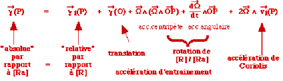
Expression des accélérations
Composition des accélérations
Il nous faut dériver par rapport au temps dans [\(R_a\)] la relation :
\(\displaystyle{\overrightarrow{v(P)}=\overrightarrow{v_1(P)}+\overrightarrow{v(O)}+\overrightarrow\Omega\wedge\overrightarrow{OP}}\)
\(\displaystyle{\overrightarrow{\gamma(P)}/[R_a]=(\frac{{d}\overrightarrow{v(P)}}{{dt}})/[R_a]=(\frac{ d\overrightarrow{v_1(P)}}{{dt}})/[R_a]+(\frac{ d\overrightarrow v(O)}{{dt}})/[R_a]+(\frac{ d}{{dt}}(\overrightarrow\Omega\wedge\overrightarrow{OP}))/[R_a]}\)
En utilisant la relation entre les dérivées temporelles et en introduisant des notations simplifiées:
\(\displaystyle{\overrightarrow{\gamma(P)}/[R_a]=\overrightarrow\gamma(P)}\)
\(\displaystyle{(\frac{{d}\overrightarrow{v(P)}}{{dt}})/[R_a]=(\frac{{d}\overrightarrow{v_1}(P)}{{dt}})/[R]+\overrightarrow\Omega\wedge\overrightarrow{v_1}(P)=\overrightarrow{\gamma_1}(P)+\overrightarrow\Omega\wedge\overrightarrow v}\)
\(\displaystyle{(\frac{{d}}{{dt}}(\overrightarrow\Omega\wedge\overrightarrow{OP}))/[R_a]=\frac{{d}\overrightarrow\Omega}{{dt}}\wedge\overrightarrow{OP}+\overrightarrow\Omega\wedge(\frac{ d\overrightarrow{OP}}{{dt}})/[R_a]}\)
\(\displaystyle{=\frac{ d\overrightarrow\Omega}{{dt}}\wedge\overrightarrow{OP}+\overrightarrow\Omega\wedge\overrightarrow v_1(P)+\overrightarrow\Omega\wedge(\overrightarrow\Omega\wedge\overrightarrow{OP})}\)
En additionnant le tout, on obtient la composition des accélérations
\(\displaystyle{\overrightarrow\gamma(P)=\overrightarrow{\gamma_1}(P)+\overrightarrow\gamma(O)+\overrightarrow\Omega\wedge(\overrightarrow\Omega\wedge\overrightarrow{OP})+\frac{ d\overrightarrow\Omega}{{dt}}\wedge\overrightarrow{OP}+2\overrightarrow\Omega\wedge\overrightarrow{v_1}(P)}\)
Remarques importantes
Pour le calcul de la dérivée du vecteur vitesse de rotation instantanée par rapport au temps, on omet de préciser le référentiel : le résultat est indépendant. En effet,
\(\displaystyle{\frac{ d\overrightarrow\Omega}{{dt}}/[R_a]=\frac{ d\overrightarrow\Omega}{{dt}}/[R]+\overrightarrow\Omega\wedge\overrightarrow\Omega=\frac{{d}\overrightarrow\Omega}{{dt}}}\)
En ce qui concerne le double produit vectoriel ; il y a lieu de calculer d'abord
\((\displaystyle{\overrightarrow\Omega\wedge\overrightarrow{OP}}){ puis }\overrightarrow\Omega\wedge(\overrightarrow\Omega\wedge\overrightarrow{OP})\)
Accélération d'entraînement et accélération de Coriolis
On appelle accélération d’entraînement \(\overrightarrow{\gamma_e}\)e vecteur
\(\displaystyle{\overrightarrow{\gamma_e}=\overrightarrow\gamma(O)+\overrightarrow\Omega\wedge\overrightarrow\Omega\wedge\overrightarrow{OP}+\frac{{d}\overrightarrow\Omega}{{dt}}\wedge\overrightarrow{OP}}\)
C'est l'accélération du point coïncidant à l'instant \(t\) avec \(P\) dans le référentiel [\(R\)]. On appelle accélération de Coriolis ou complémentaire le vecteur \(\overrightarrow{\gamma_c}\)
\(\displaystyle{\overrightarrow{\gamma_c}=2\overrightarrow\Omega\wedge\overrightarrow{v_1}(P)}\)
\(\overrightarrow\gamma_c\) est liée au mouvement de \(P\) dans [\(R\)]; c'est un vecteur perpendiculaire au plan . En particulier l'accélération de Coriolis est nulle si \(P\) est fixe dans [\(R\)].
En résumé:
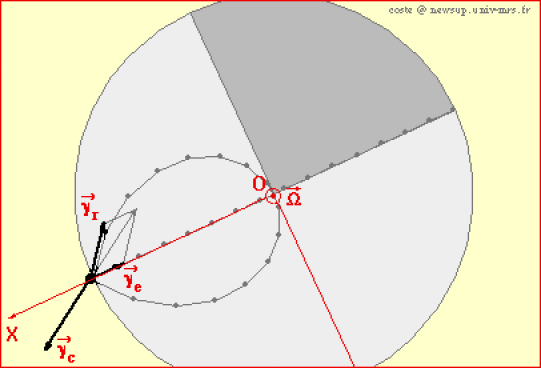
Par rapport au disque en rotation, le point a une accélération relative qui représente la variation de sa vitesse relative.
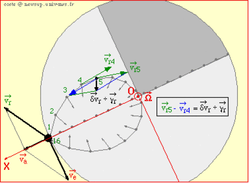
Dansla simulation suivante, l'accélération du point est nulle par rapport au référentiel du laboratoire. Par rapport au disque en rotation, le point a une accélération relative.
Remarque:
Les mouvements s'observent par rapport à différents référentiels :
le référentiel noté \((a)\) qui peut servir de référence à tout mouvement est parfois appelé "Référentiel absolu", mais cette dénomination est incorrecte car il n'y a pas de critère d'absolu.
le référentiel noté [\(R\)], qui est animé par rapport à [\(R_a\)] d'un mouvement a priori quelconque.
[\(R\)] est parfois appelé "Référentiel relatif", ce qui est redondant :
Tous les référentiels sont en mouvement : ils sont donc tous "relatifs".